Harrison Espino, Robert Bain, Jeffrey Krichmar
University of California, Irvine

Mapping traversal costs in an environment and planning paths based on this map are important for autonomous navigation. We present a neurorobotic navigation system that utilizes a Spiking Neural Network (SNN) Wavefront Planner and E-prop learning to concurrently map and plan paths in a large and complex environment. We incorporate a novel method for mapping which, when combined with the Spiking Wavefront Planner (SWP), allows for adaptive planning by selectively considering any combination of costs. The system is tested on a mobile robot platform in an outdoor environment with obstacles and varying terrain. Results indicate that the system is capable of discerning features in the environment using three measures of cost, (1) energy expenditure by the wheels, (2) time spent in the presence of obstacles, and (3) terrain slope. In just twelve hours of online training, E-prop learns and incorporates traversal costs into the path planning maps by updating the delays in the SWP. On simulated paths, the SWP plans significantly shorter and lower cost paths than A* and RRT*. The SWP is compatible with neuromorphic hardware and could be used for applications requiring low size, weight, and power.
Methods
Model
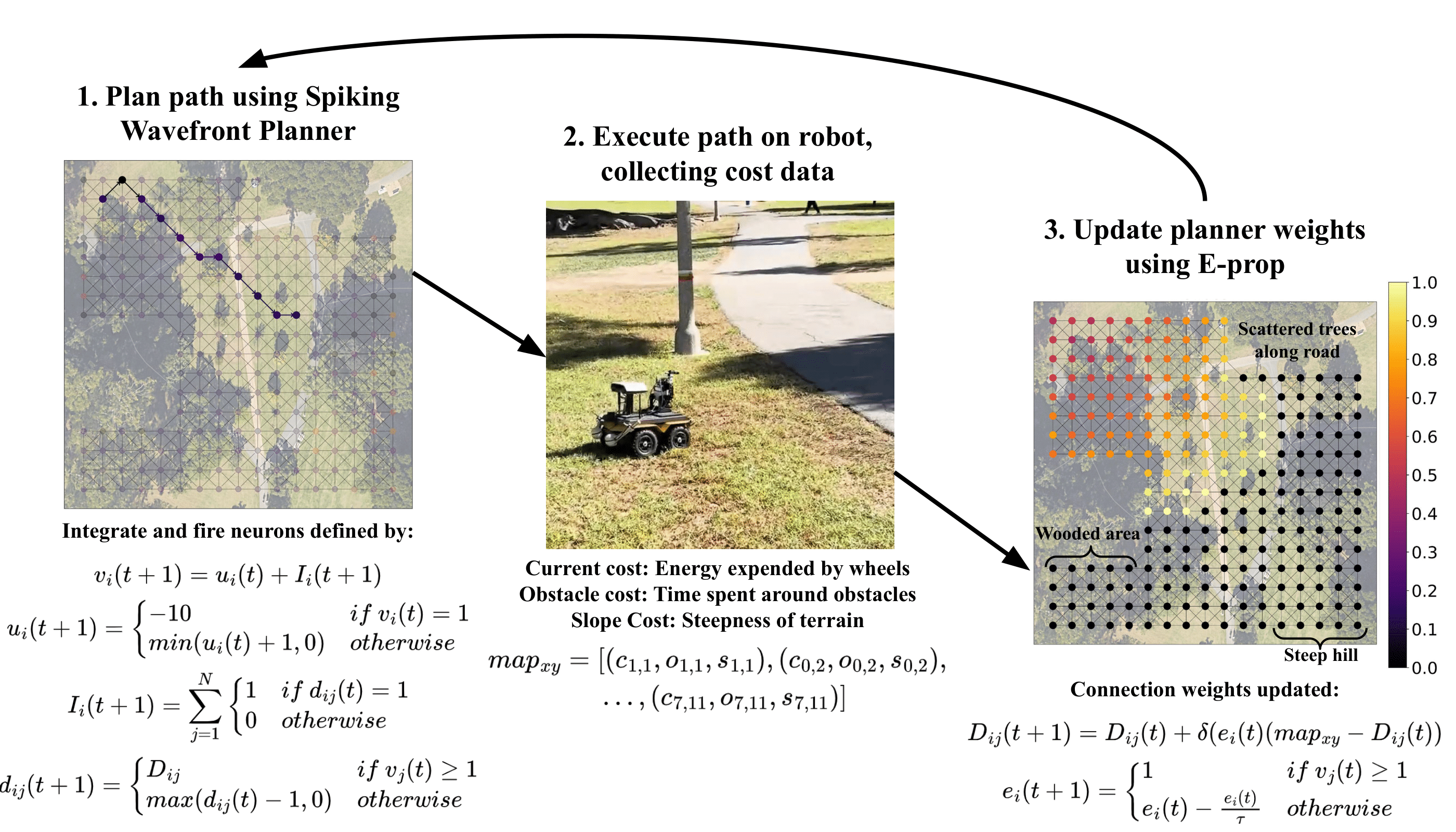
Our navigation model is inspired by experience-dependent axonal plasticity and place cells in the hippocampus. Each neuron represents a location in space, where connections between units represent the ability to traverse between them. Connections have learnable “delay” values which slows the transfer of signals between neurons. To plan a path, a signal is sent from the neuron at the robot’s current location, which propagates to it’s neighbors. This is repeated until the signal reaches the goal neuron, at which point the origin of the signal is recursively traced to determine the path.
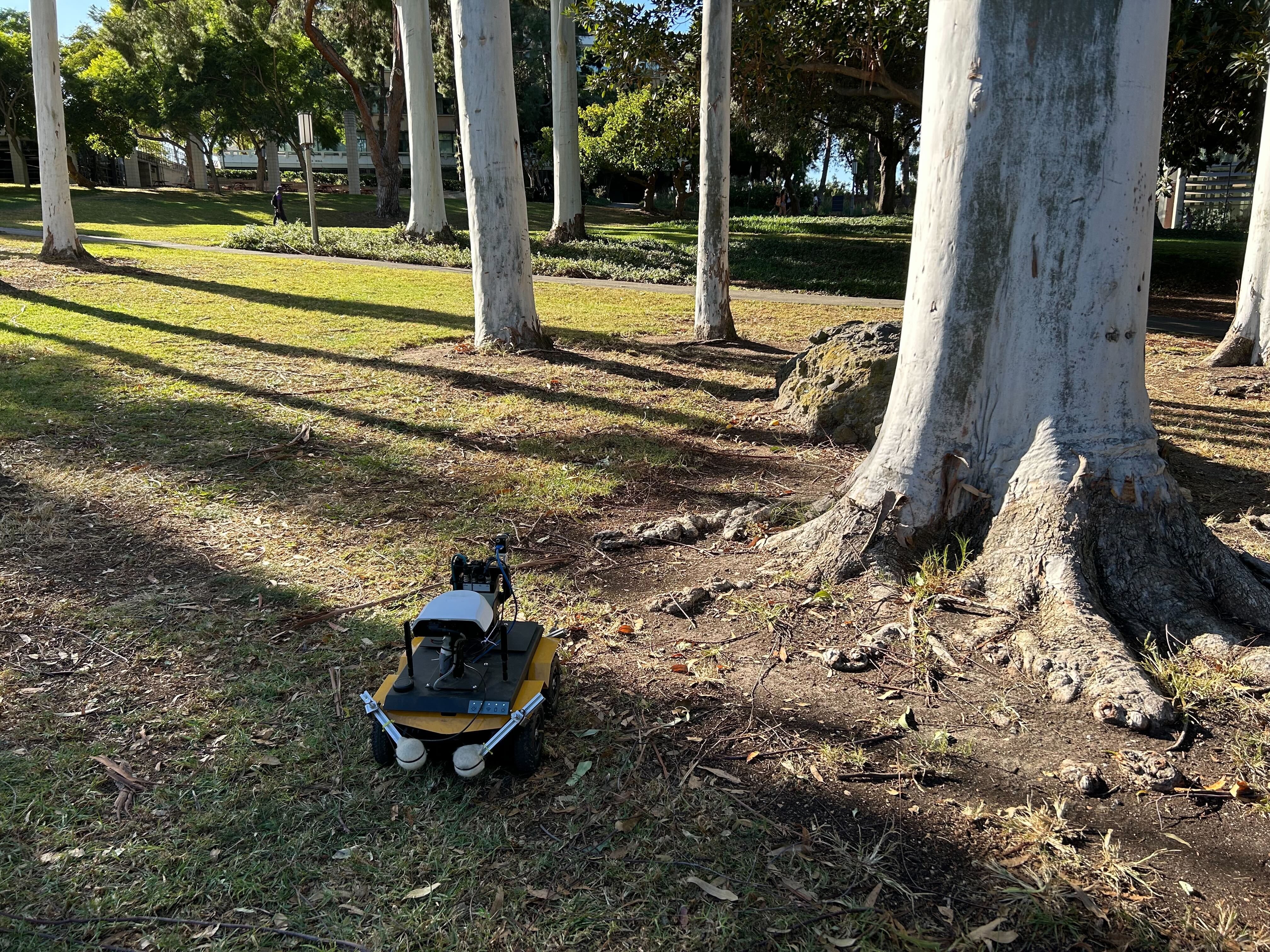
Environment
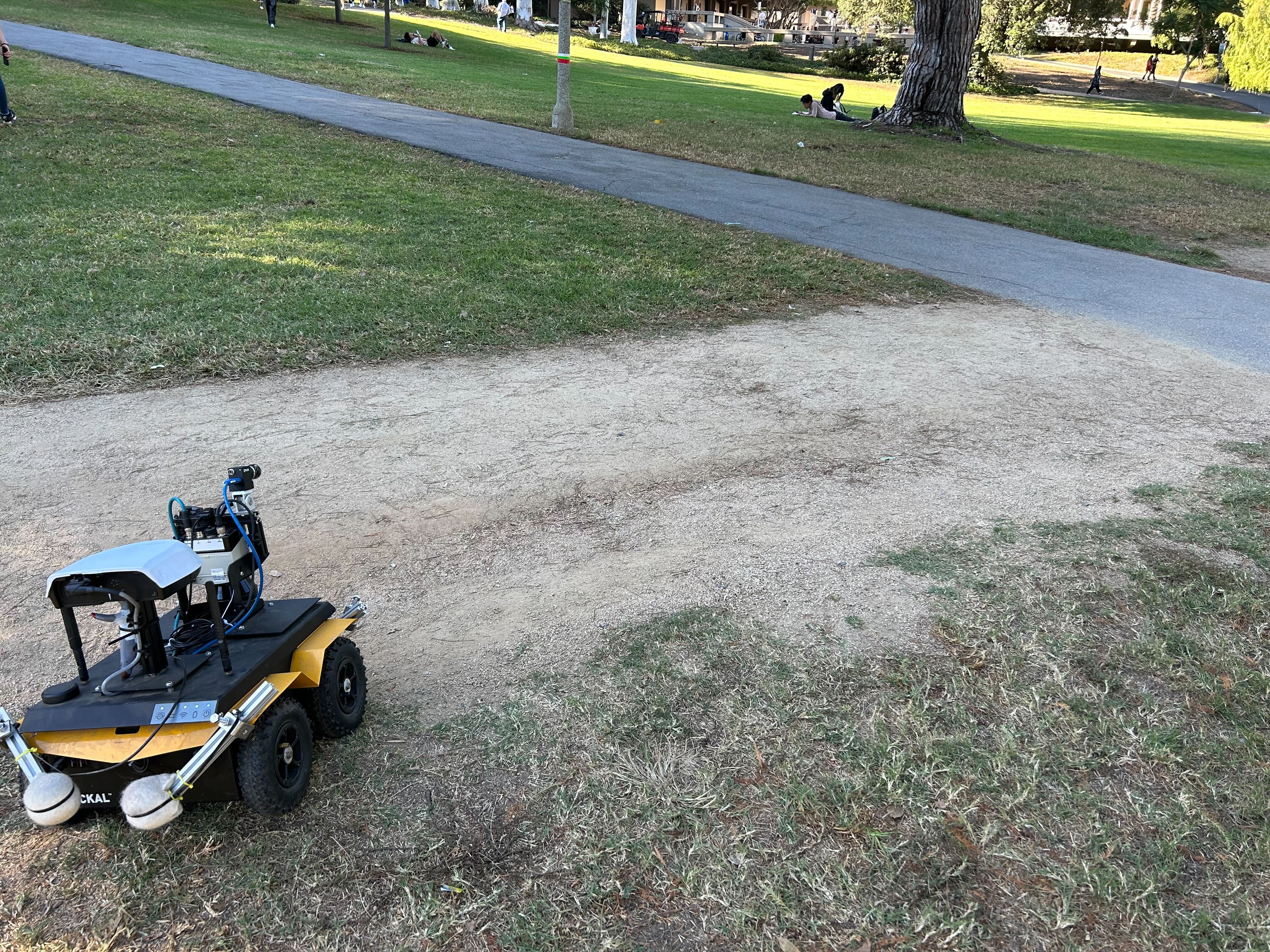
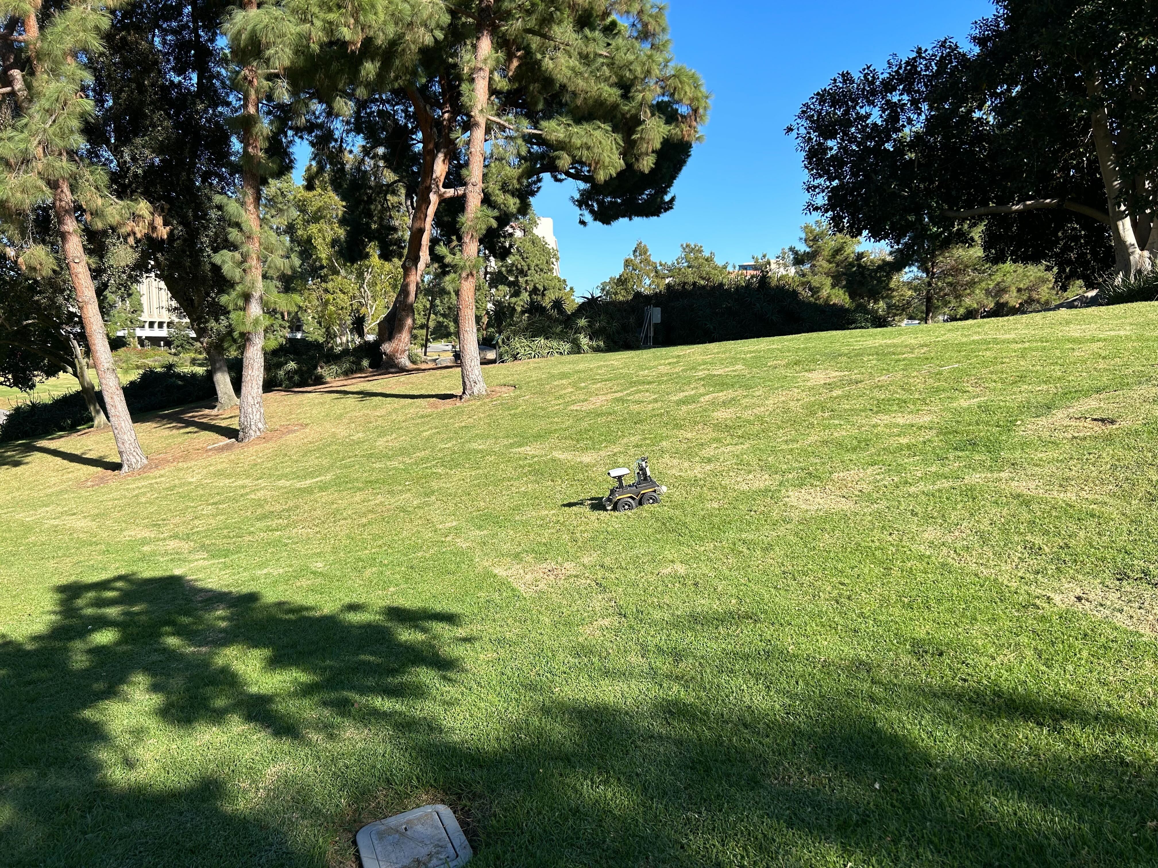
We test our model in Aldrich park, a park in the middle of the University of California, Irvine with varied terrain in the form of dirt and asphalt roads, trees, benches, and sloped hills. The robot explored this environment autonomously for 12 hours. While exploring, the robot measured the current drawn by the wheels, the time spent in the presence of obstacles, and the slope of the terrain to train the model.
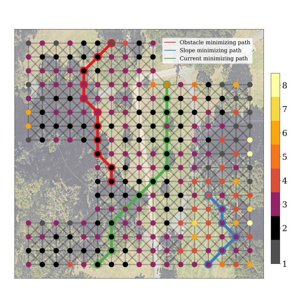
Learned Map
After 12 hours of autonomous navigation, the robot learned the map below. Nodes are colored according to the mean of incoming delay values. When minimizing obstacles, the robot avoided trees and benches. When minimizing current, the robot took a straight path, avoiding changes in terrain. When minimizing slope, the robot avoided the steep hill.
Path Planning with the Trained Model
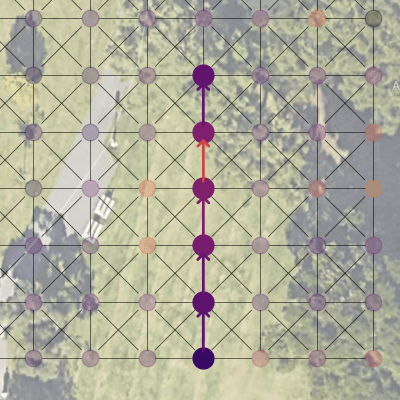
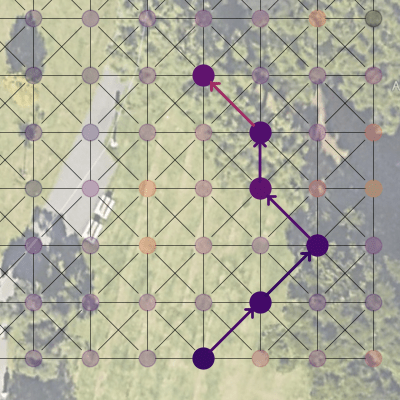
With the trained model, the robot learned to optimize its path according to the cost chosen to minimize. Here, whereas the naive solution would be to travel straight to the destination (left), the robot chooses to traverse up the hill and back down to avoid sloped terrain (right).

Naive Model
Trained Model
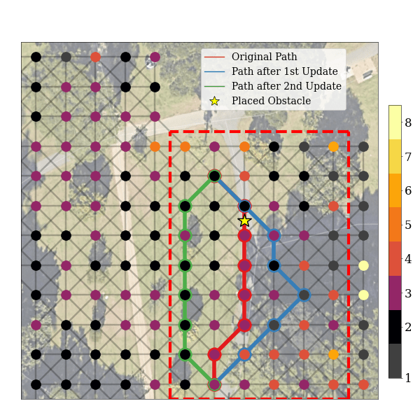
Adapting to Changes in the Environment
Our model also rapidly adapts to changes in the environment. We place an obstacle in front of the learned robot’s initial route, which travels along the road. After a single model update, the robot adapted to this change, instead taking a new route around the obstacle on the road. After a second update, the final route traveled across the grass field.